How to work in Microsoft Excel. How to write a formula in Excel: basics, most needed formulas. Pobudova graphs and diagrams

In another part of the Excel 2010 for beginners cycle, you will learn how to connect the middle of a table with mathematical formulas, add rows and columns to a ready-made table, learn about the autofill function and much more.

Enter

In the first part of the series “Excel 2010 for beginners,” we learned the basics of Excel, learning how to create basic tables with it. Strictly speaking, on the contrary, it is simple and, of course, the possibilities of this program are much wider.

The main advantage of electronic tables lies in the fact that besides data, you can connect mathematical formulas with each other. Then, when you change the value of one of the interconnected data, the other data will be re-corrected automatically.

In this part, we will figure out what benefits such possibilities can bring to the table of budget expenditures that we have already created, for which we will have to learn how to put together simple formulas. We also know about the function of autofilling the middle and find out how you can insert additional rows and columns into the table, as well as combine items into it.

Vikonanny of basic arithmetic operations

By creating basic tables, Excel can be used to add arithmetic operations in them, such as addition, substitution, multiplication and subdivision.

To display the layouts in any middle of the table, it is necessary to create it in the middle to put it simply formula, which is always obliged to begin with a sign of zeal (=). To determine the mathematical operations in the middle of the formula, the primary arithmetic operators are used:

For example, it is obvious that we need to add two numbers - “12” and “7”. Place the mouse cursor in any box and select the next line: “=12+7”. After completing the entry, press the “Enter” key and the calculation result will appear in the box - “19”.

In order to find out what is the right way to replace the middle - a formula or a number - it is necessary to see and admire the series of formulas - the area that lies just above the names of the formulas. In our version, it displays the formula that was carefully administered to us.

After carrying out all operations, pay attention to the result of the subdivision of numbers 12 by 7, whichever we do not target (1.714286) and replace a lot of numbers after the coma. For most types, such precision is not required, and such long numbers will no longer characterize the table.

To correct this, see a comment with a number in which you need to change a number of tenths digits after the entry on the deposit. Golovna in the group Number select a team Change the capacity. Pressing the skin on the button reveals one sign.

Livoruch as a team Change the capacity There is a button that selects the reverse operation - increase the number of characters after the number to display more precise values.

Formula folding

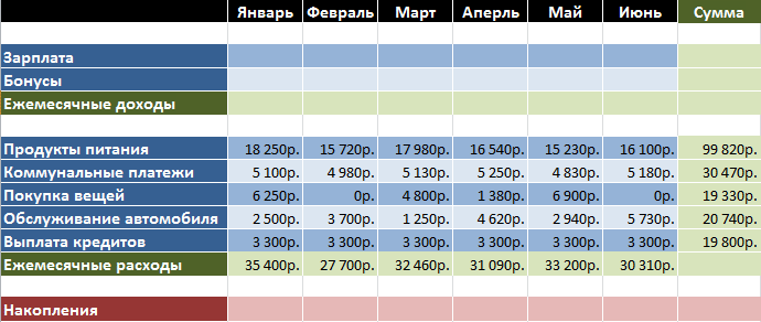
Now let's go back to the table of budget videos that we created in the first part of this cycle.

At the moment, she has recorded thousands of special expenses for specific items. For example, you can find out how much was spent on groceries or on car servicing. And the whole waste of millions of dollars in expenses is not indicated here, although these are indications for the rich and the most important. Let's correct this situation by adding a row at the bottom of the table “Thousandths of expenses” and expanding its values.

To calculate the total payment for the sum in the middle B7, you can write the following expression: “=18250+5100+6250+2500+3300” and press Enter, after which you will enter the calculation result. This is just a simple formula, the folding of which is in no way different from calculating on a calculator. It’s just a sign to be put first and foremost, but not at all.

And now you realize that when you enter the value of one or several articles of expenditure, you are forced to make amends. In this case, you will have to collect not only the data in the middle from the assigned expenses, but also the formula for calculating the total expenses. Of course, it’s not easy at all, and that’s why in Excel, when formulating formulas, it’s often not specific numeric values, but addresses and ranges of frequencies.

Looking at the price, let's change our formula for calculating total monthly expenses.

For box B7, enter the sign one (=) and... instead of manually entering the values ​​of box B2, click on it with the left mouse button. After this, a dotted vision frame will appear next to the box, showing what value has been lost in the formula. Now enter the “+” sign and click on the middle B3. Then try the same with the middles B4, B5 and B6, and then press the ENTER key (Enter), after which the same sum values ​​​​will appear as in the first step.

See the new commercial B7 and see a series of formulas. It can be seen that the replacement of numbers is the value of the middles, and the formula contains their addresses. This is an extremely important point, because we only developed the formula not from specific numbers, but from the meaning of the middles, which can change over time. For example, if you now change the amount of expenses for the purchase of speeches from Sichna, then the entire thousand-thousandth amount of expenses will be reinsured automatically. Try it.

Now it is acceptable that it is necessary to calculate not five values, as in our example, but one hundred and two hundred. As you understand, it is not easy to use the method of motivating formulas in this case. In this case, it is better to quickly use the special “AutoSum” button, which allows you to calculate the amount of several middles between one column or row. In Excel, you can enter not only sums of columns, but also rows, so you can use them to calculate, for example, waste expenses on food products for food.

Place the cursor on the empty button on the side of the required row (our type has H2). Then press the button Suma on deposit Golovna in the group Editing. Now let’s go back to the table and wonder what happened.

The company we selected had a formula with an interval of midpoints, the values ​​of which need to be summed up. At this sound, a dotted vision frame appeared. Only this time it frames not just one cell, but the entire range of objects that need to be secured.

Now let's marvel at the formula. As before, initially there is a sign of jealousy, but now it is followed by function"SUM" - the formula is indicated behind, which calculates the folded value of the meanings of the middles. Immediately after the function there are arms drawn around the address of the clients, the meanings of which must be included, the name formula argument. Please note that the formula does not indicate all the addresses of the companies, but only the first and the remaining ones. The double dot between them means what is indicated range klitin from B2 to G2

After pressing Enter, the selected middle will display the result, and on the button's options Suma will not end. Click on the arrow next to it and a list will open where you can use functions to calculate average values ​​(Average), number of input data (Number), maximum (Maximum) and minimum (Minimum) values ​​.

Well, in our table we praised the total expenditure for the whole day and the total expenditure for food products for the sum. In this case, we created this in two different ways - from the beginning with the formula in the formula, the address of the middle, and then the function and range. Now, it’s time to finish the disbursement for the midgets that you have lost, having recovered the waste behind the bars of months and articles of expenditure.

Automatic filling

To sort out the money that you have lost, you can quickly use one miraculous feature of the Excel program, which is its ability to automate the process of filling in the middle with systematized data.

Sometimes in Excel you have to enter similar data of the same type, for example, days of the year, dates and serial numbers of rows. Do you remember that in the first part of this cycle at the top of the table we introduced the name of the month for the skin? In fact, it was not at all necessary to enter this entire list manually, but the program can do it for you in many ways.

Let's look at all the names of the months at the head of our table, except for the first one. Now see the box with the inscription “Cross” and move the mouse indicator near the right and bottom corner so that it takes the shape of a cross, which is called waste marker. Press the left mouse button and drag the right mouse button.

A prompt will appear on the screen to tell you the values ​​that the program is going to insert into the slot. Our guy has a whole life. When you move the marker all the way down, it will change to the names of other months to help you figure out where you need to go. When the button is released, the list will be filled in automatically.

Of course, Excel does not always correctly “understand” the need to fill in the steps, the sequence fragments can be quite different. It is clear that we need to fill the row with the same numerical values: 2, 4, 6, 8 and so on. If we enter the number “2” and try to move the autofill marker to the right, then it will appear that the program replies as soon as it arrives, and in the other middle, insert the value “2” again.

In this case, the supplement must be given much more data. For this purpose, enter the number “4” in the right-handed center. Now you can see that the mouse has been filled in and move the cursor at the bottom right corner of the view area again so that it takes the shape of a view marker. By moving the marker down, it is clear that the program has now understood our sequence and shows the required values ​​in the tooltips.

Thus, for complex sequences, before completing the autofill, you must independently fill in a number of middles so that Excel correctly calculates the original algorithm for calculating their values.

Now let's put this entire program into our table so that we don't have to enter formulas manually for clients that we've lost. Right away you can see a small bag with a bag already covered (B7).

Now “snap” the lower right corner of the square with the cursor and drag the marker to the right to the middle G7. After you release the key, the program itself will copy the formula from the specified middle, automatically changing the addresses of the clients to be located in the expression by inserting the correct values.

If you move the marker to the right, as in our fall, or down, then the middle ones will appear in the order of increasing, and to the left or up, in the order of falling.

There is also a way to complete the row behind the additional stitch. It is necessary to quickly calculate the amount of expenditures for all expenditure items (section H).

You can see the range that you need to fill in when you start entering the data. Then on deposit Golovna in the group Editing pressing the button Save And we select filling directly.

Addition of rows, additions and combination of middles

In order to get more practice from the folded formulas, let's expand our table and immediately learn a number of basic formatting operations. For example, we will add up to the tax part of the income statement, and then we will decompress possible budget savings.

It is acceptable that the profitable part of the table of roztashovuvatimes is for the beast above the videotape. For this purpose we have to insert a number of additional rows. As always, you can do it in two ways: vikory commands on the page or in the context menu, whichever is simpler and faster.

Right-click on the mouse in the middle of another row and select a command from the menu Insert..., and then at the window - Add a row.

After inserting a row, pay attention to the fact that it is inserted above the selected row and changes the format (color of the background of the middles, adjustment of the size, color of the text, etc.) to the row that is above it.

If you need to change the formatting, please press the button after inserting Addition parameters, which will automatically appear in the lower right corner of the selected store and select the required option.

Using a similar method, you can insert columns into the table that will be placed left-handed from the center and around the middle.

Before speaking, if the result is a row or a stop after the insertion has ended in an unnecessary place, they can be easily deleted. Right-click on any business to locate the object that is visible, and select the command from the menu vidality. When finished, indicate what needs to be removed: row, side or middle.

On the page for additional operations you can click on the button Paste, roztashovana from the group Middles on deposit Golovna, and for the sake of clarity, the same team in the same group.

For our example, we need to insert five new rows at the top of the table immediately after the header. To do this, you can repeat the additional operation several times, or you can, having selected it once, press the “F4” key, which repeats the remaining operation.

The result, after inserting five horizontal rows at the top of the table, brings it to the following view:

We removed the unformatted rows in the table on purpose in order to strengthen the income, data and storage part of one type by writing separate headings in them. Before we do this, let’s perform one more operation in Excel - sharing of middles.

When a number of equal middles are combined, one is created that can be used in several rows and rows. In this case, the middle middle becomes the address of the uppermost middle of the general range. Whatever the case, you can break the middle again, but you won’t be able to break the klitin, which has never been eaten.

When merging the middle, only the data from the top left is saved, and the data from all other combined middles will be deleted. Remember this and start by understanding the details first, and then enter the information.

Let's go back to our table. In order to write headings in large rows, we only need one middle, at a time when the smells add up to eight. Let's get this straight. See all the middle rows in another row of the table and on the tab Golovna in the group Virivnyuvnya click on the button Combine and place in the center.

After finishing the command, all the visible boxes in a row are combined into one big box.

Using the merge button, there is an arrow, pressed on a menu with additional commands that allow you to: merge centers without central alignment, combine groups of centers horizontally and vertically, as well as suvati ob'ednannya.

After adding headings, as well as filling out rows: salary, bonuses and thousands of income, our table began to look like this:

Visnovok

First of all, let's explore the remaining row of our table, quickly removing the knowledge in this article, calculating the value of the middle that follows such a formula. In the first month, the balance is formed due to the significant difference between the income withdrawn for the month and illegal expenses from the new person. And the axis of the other month to this difference is added to the balance of the first, so that we know how to accumulate the reserves. Disbursements for the coming months will follow the same scheme - the accumulations for the previous period will be added to the current monthly balance.

Now let's translate this structure into complex Excel formulas. For today (commercial B14) the formula is even simpler and will look like this: = B5-B12. And the axis for the center C14 (lutiary) can be written in two different ways: “= (B5-B12) + (C5-C12)” or “= B14 + C5-C12”. In the first phase, we renew the balance of the previous month and then add the current balance to a new one, and in the other, the formula includes the result of the previous month. Of course, choosing another option to create a formula in our case is much better. If we follow the logic of the first option, then for the birch structure there will already be 6 middle addresses, for the knit - 8, for the grass - 10 and so on, and if you choose another option, there will be three of them .

To fill the centers from D14 to G14, the possibility of their automatic filling is stagnated, as they were prevented from running out of sums.

Before speaking, in order to verify the value of the sum of the accumulated cash on the red, which is in the G14 client, in the middle of H14, you can enter the difference between the total amount of monthly income (H5) and monthly expenses (H12). As you can imagine, the stench is strong.

As can be seen from the remaining layouts, the formulas can be modified not only to the addresses of the adjacent parts, but also to some others, regardless of their placement in the document or their affiliation with one or another table. Moreover, you have the right to link the marks that are found on different arches of the document and in different books, and we’ll talk about them in the next publication.

And the axis is our sub-table with the following rows:

Now, for sure, you can independently continue to do this by inserting additional items, expenses and income (rows), and adding new months (stacks).

In the following material, we will talk in more detail about the functions, understand the concepts of basic and absolute instructions, and be sure to master a number of basic elements, the editing table, and much more.

The Microsoft Office office suite includes the Excel spreadsheet processor. A special feature of the Excel spreadsheet is the automatic layout of data from previously prepared formulas. p align="justify"> Electronic tables are mainly used for working with numerical data, but textual values ​​can also be processed in them.

Getting to Know Spreadsheets

The skin cell of the electronic table is called the middle. May have the most powerful designation – it’s my name. As a rule, the name is first set to the name of the column and the row number on the webbing that has been sewn. For example, G5, E8.

The main types of data for processing in electronic tables, which can be processed and recorded in tables, are numbers, text and formulas.

Numbers can accept goals and shot values.

text The sequence of characters, including numbers, is important.

Formula This is a record that begins with the sign "=" (equally), which contains the addresses of middles, signs of arithmetic operations, numbers and functions.

A document created in Excel is called a book and can contain a number of labels, which are placed at the bottom of the window. When saving a workbook in Excel, all entries will also be saved in a single file.

The external appearance of the interface for all add-ons included in the Microsoft Office package practically does not change, so if you have mastered one of them, you can easily navigate Excel.

Familiar with the program interface. On the little one below the upper part of the window block No. 1(Visions in red color) Place the left button on the quick access panel, in the middle the name of the stream file Book1 is displayed, right-handed, not shown on the little one, standard window control buttons.

New look for the Excel 2016 interface

Block No. 2(In the same color) place the row of tabs with tools.

Block No. 3(shown in green color) You can place a field in which the name (address) of the active center is displayed. Then there are three buttons in the formula editing mode:

• cross - visible from introduction into the production line - removed instead;
• checkmark - complete editing instead of compilation;
• Fx – the function master's tool for filling in the middle with the imported functions of the table processor.

The third field (double) is used for displaying instead of the active middle or division of the formula.

In the active middle, the result of the breakdown by formula is automatically displayed, which instead of the formula will be visible in block No. 3. There you can edit the formula.

Block No. 4(Violet color) Brush the work area (table). The table entries are designated by Latin letters in alphabetical order. The rows are numbered in Arabic numerals per row. At the bottom of the work area, shortcuts for arches are displayed, which can be added using the plus button.

Block No. 5 Place a row on the right side of which there are expanded buttons with table display modes: initial, side layout, side and scale instead of arch.

Video: Adding numbers in Excel

How to create a formula in Excel

Let's take a look at the simple calculations in the electronic table. We model the forming of a receipt for a cash register at a store.

Formation of a purchase receipt

You can clearly see the number of purchases, the number of products, their quantity, the price per unit and the variety of each product. All calculations are carried out using the formulas in section E and in the middle E1. Let's figure out what the formulas are and how the structure is derived from them.

Calculation of product costs in Excel

In the middle E5 the formula is given =C5*D5 which multiplies the number of units of a product and the price per unit of the product. For some rows there will be similar formulas, only they will change the part of the address in the middle, which indicates the row number. For example, chocolate is in the ninth row of the table and the formula for the distribution of goods in commerce E9 sure enough I see it =C9*D9. Formulas can be entered manually for the skin row, or you can copy the formula from the copy E5 down to E9(Inclusive).

Copying formulas in Excel

Copy. Finish editing the flow formula by pressing the button Enter on the keyboard. Click on the box to replace the formula. Place your mouse at the bottom right corner of the visible box. As soon as the user switches to the black plus sign, press the left button of the mouse and, without releasing it, drag the frame down onto the box E9. The formula will be inserted into the indicated account and the calculation result will be automatically displayed in them.

When copying, the addresses of the middles in the formulas are changed accordingly to the numbers of the rows that will have them. This change of address is called the principle of portable addressing.

To expand the size of the pouch, it is necessary to include in the middle of the range E5:E9. For whom in the middle E10 let's write down the formula =E5+E6+E7+E8+E9.

To pay for the payment to the commercial office E12 let's write the formula = E11-E10. At the middle E11 Enter the amount of cooking.

The calculation table is ready. Now, when you change the quantity and price of a product, their value will be re-insurance automatically.

Utility services: electricity, gas, water

To record expenses for utility bills, you can create a similar table. If you would like to create such an electronic table, write your thoughts in the comments. Do you want to admire the file right away? Your request for downloading the file Utility services

Dear Reader! You looked through the article to the end.
How much did you take away for your nutrition? Write a few words in the comments.
Because they didn’t know the subtypes, tell me what you were joking about.

This will make it easier for you to work with tables and numerical expressions that automate them. Who can be reached for additional program tools and other functions. Let's take a look at the best ones.

Due to the wide functionality of the program, the developer is not always aware of the possibilities of how to easily interact with the wealth of Excel tools. Below we will tell you about 10 of the most important functions that can be useful for various purposes, as well as information about them.

Function "VLOOKUP"

One of the most popular functions of Microsoft Excel is "VLOOKUP". Once entered, you can drag the values ​​from one or more tables to another. If the search is carried out only in the first column of the table, then when changing the data in the table-jerel, the data of a similar table are automatically formed, in which they can be added around the expansion. For example, information from the table, which contains price lists for goods, can be used to break down the displays in the table about purchasing obligations in penny terms.

VVR is launched by the operator insertion path "VVR" h "Maistri functions" in the middle where the data may appear.

In the window, after running this function, you need to specify the address of the middle or the range of middles, the data will be adjusted.

Table entries

Another important function of the Excel program is the creation of a summary table, which ensures the grouping of data from other tables according to different criteria, the arrangement of different structures with them (summation, multiplication, division, etc. ), and the results are displayed in a table. In this case, there is a wide range of possibilities for customizing the fields in the table.

Created on the deposit "Insert" pressing on the button, that’s what it’s called "The table has been created".

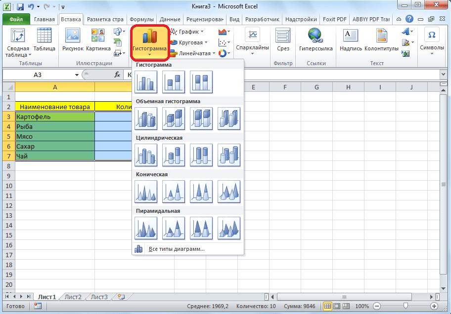
Creation of diagrams

To visually display the data placed in the table, manually use diagrams. They are often used for creative presentations, scientific writing, and for other purposes. Excel provides a wide range of tools for creating different types of diagrams.

To create a diagram, you need to see a set of data points that you want to visually represent. Then, while on deposit "Insert", Select on the page the type of diagrams that you think is most suitable for achieving the goal.

More precisely, the adjustment of diagrams, including the installation and naming of axes, is carried out in a group of tabs "Working with diagrams".

One of the types of diagrams is graphs. The principle is the same as in other types of diagrams.

Formulas in Excel

p align="justify"> For working with numerical data in the program, you are allowed to use special formulas. With their help, you can carry out various arithmetic operations with data in tables: adding, subtracting, multiplying, subdividing, adding to the root, etc. To formulate the formula, you need to put a sign in the middle where you plan to display the result. «=» . After this, the formula itself is introduced, which can be composed of mathematical signs, numbers and the address of the middle. To enter the address of the merchant from which the data for packaging is taken, just click on it with the mouse and its coordinates appear in the merchant to display the result.

Excel is also easy to use as a basic calculator. For this purpose, in a series of formulas or in any middle, simply introduce mathematical expressions after the sign «=» .

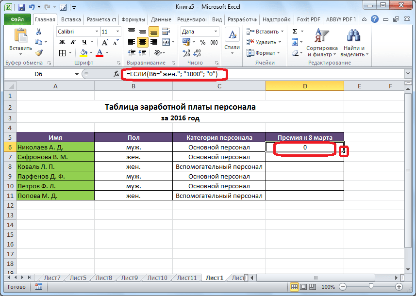
Function "YAKSCHO"

One of the most popular functions that are used in Excel is "YAKSCHO". It gives you the ability to set one result in the middle of a specific mind and another result for a different reason. The syntax looks like this: YAKSCHO (logical expression; [result is true]; [result is false]).

Operators «І», "ABO" and the embedded function "YAKSCHO" The similarity of several minds or one of many minds is set.

Macros

Using additional macros, the program records a list of song actions, and then they are created automatically. It is worth saving an hour from the great number of similar robots. Macros are recorded by storing your actions in the program via the dedicated button on the page.

Recording macros can also be done using a special editor using Visual Basic markup.

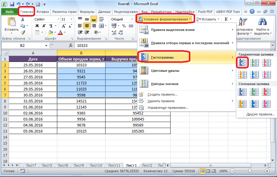
Washroom format

To see the song data, the table has a mental formatting function, which allows you to adjust the rules for seeing the middle. The most intelligent formatting is allowed to be displayed like histograms, color scales, or a set of icons. You can get to it through the tab "Golovna" from the views of the middles that you choose to format. Further in the group of tools "Styles" press the button with the name "Umovne formatuvannya". Then you will not be able to select the formatting option that you think is most suitable.

The formatting will be changed.

"Reasonable" table

Not all developers know that a table, simply framed or bordered, is treated by Excel as a simple area of ​​\u200b\u200bcompositions. You can use the program to type this data as a table through reformatting. It’s easy to work out: initially you can see the required range of data, and then continue on the deposit "Golovna", click on the button "Format the table". A list will appear with different options for design styles, and select the one that suits you.

The table is also created by pressing the button "Table", as it was retouched on the deposit "Insert", having previously seen the song area of ​​the arkush of data.

The editor will treat the sequence of images as a table. As a result, for example, if you enter any data in the spreadsheet between the payment table, they will be automatically included before it. In addition, when scrolled down, the cap will remain firmly within the viewing area.

Select parameter

Using the additional function of selecting parameters, you can select output data that produces the desired result for you. Go to tab "Dani" and press the button “Analysis of “what is it like””, added to the toolbox "Robot with money". Select item from the list "Select parameter...".

The parameter selection window appears. In the field "Install in commerce" You are responsible for sending the mail to your mailbox in order to obtain the required formula. In the field "Significance" It is the end result that you want to reject that is to blame. In the field “The changing significance of the business” insert the coordinates of the store with the adjusted values.

Function "INDEX"

Possibilities that the function provides "INDEX", I think the functions are close to the capabilities "VVR". It also allows you to search for data in a value array and rotate it using the specified value. The syntax looks like this: INDEX (middle_range; row number; column number).

This is far from a complete change from the existing functions available in Microsoft Excel. We paid respect only to the most popular and most important of them.

Statistics lovers often complain that they do not like to calculate and calculate. They must calculate, analyze ready-made figures and maintain a scrupulous attitude. Now, with the advent of electronic processors, such people are faced with indispensable opportunities. There is nothing simpler than to conduct statistical and other appearance in the Excel program from the Microsoft office package.

Basic concepts and functions

When starting to work in Excel with tables, it is important for beginners to grasp the basic concepts and principles of working with this program. Like a Windows program, Excel has a traditional interface for such programs.

The menu includes sections that control all components of the Microsoft Office package: header, insertion, side layout, view, review. The tabs that govern this program: formulas and data.

The external appearance of the working area of ​​presentations is similar to that of the page, which is divided into sections. The center has its own number and coordinates. For this purpose, the largest column of numbering and the first top row have their numbering in the form of Latin letters. The coordinates of the box are indicated by the web of the vertical line with the letter and the horizontal line with the number.

The skin center is a collection of data. What can you do: numbers, text, formula for calculation. To any extent, it is possible to establish the differences in power and types of data formatting. For this purpose click on the market with the right mouse button. From the menu, select the “Format in Middle” section.

All the middles are gathered around the leaves. At the bottom of the program window there are labels with the names of the arches. Wrap up Sheet1, Sheet2 and Sheet3, and make a label to create a new sheet. All sheets can be renamed to the authorities. To do this, you need to move the cursor over the shortcut and press the mouse button to the right. From the menu, select an additional command. This can also be deleted, copied, moved, pasted, grabbed and stolen.

Due to the large number of items in one Excel file, such files are also called books. Books are given names and can be easily saved by sorting them into folders.

Created table

Basically, you need to know how to work with Excel tables, so it’s important for everyone to learn how to work with tables in Excel. In contrast to their Word counterparts, Excel offers a number of significant advantages:

1. You can carry out refreshments and calculations.
2. They can sort the data according to selected criteria. Most often for growth or for decline.
3. They can be linked to other sides and work dynamically, so that when you change the data in the linked fields, the data in the other linked fields is changed.
4. p align="justify"> Information from such data banks can be mined to create histograms, graphs and other interactive elements, which is very useful for presenting data online.

These are not all the advantages of Excel documents. The actual creation of fields that are calculated is extremely simple in Excel. The required steps to draw such an object are:

Having tried to create one small tablet, any kind of teapot can easily create objects of different configurations in the same way. When dealing with them, there are many who are aware of other corrosive powers of Excell elements and are happy to use them for their needs.

Calculation using additional formulas

Young Asians who have mastered how to work with tables in Excel can then become self-sufficient. Moreover, in addition to the Ordovo twin city, Excel’s collection of data provides endless possibilities for various calculations. It is enough to acquire a little skill, how to insert formulas and carry out calculations in many objects.

To create a field that is calculated in Excel, just see the mark and press the “=” sign on the keyboard. After this, the calculation values ​​that are located in any middle of this table become available. To compress or expand the values, see the first middle, then put the required number sign and see the other middle. After pressing Enter, the result of the calculation will appear in the middle for the selected item. In this manner, it is possible to carry out various calculations of any middle items that indicate the ability to calculate what is being carried out.

To make it easier to work with tables in Excel, create numerical formulas. For example, finding the sum of how many middles there are in one row or one column is the formula “sum”. To do this, it is enough after selecting the box and pressing on “=” in the row above the top row of the arch on the left side, select the required formula from the list, which appears after pressing on the small jersey in the box with formulas.

Having learned to profit from this simple technology, many statistics lovers have become comfortable with the masses of large calculations and inescapable benefits, like people in power, and daily at calculating machines.

In the third part of the materials “Excel 2010 for cobs” we will talk about algorithms for copying formulas and the system for accelerating corrections when they are folded. In addition, you will learn what these functions are, as well as how to present data and calculate the results in a graphical view using additional diagrams and sparklines.

Enter

In another part of the “Excel 2010 for beginners” series, we learned how to format a table, for example, adding rows and columns, as well as combining rows. Finally, you learned how to calculate arithmetic operations in Excel and began to create simple formulas.

To begin with this material, let’s talk a little more about formulas - obviously, how to edit them, let’s talk about the notification system for errors and the tools for acknowledging errors, and we will also learn about the use of some algorithms in Excel for copying and transferring displacement of formulas. Then we will learn about another important concept in spreadsheets – functions. Finally, you will know that with MS Excel 2010 you can present data and draw results in a graphical form, using charts and sparklines.

Editing formulas and the system for fastening milk mixtures

All formulas that are in the middle of the table can be edited at any time. To do this, you just need to see the formula box and then click on the row of formulas above the table, where you can immediately make the necessary changes. If it is more convenient for you to edit instead of directly in the world itself, then click on it.

After finishing editing, press the Enter or Tab keys, then Excel will re-arrange the changes and display the result.

It often happens that you have entered the formula incorrectly, or after changing it instead of one of the middle steps, which is used by the formula, there will be a reduction in the calculations. With this type of error, Excel will immediately inform you about it. Order behind the cage, where Milk’s viraz will take place, a sign of a hail will appear, in the yellow rhombus.

In many cases, the additions will not only inform you about the presence of the mistake, but also those that are not formed correctly.

Decryption of pardons in Excel:

• ##### - the result of the formula is that the vikory value of the date and time has become a negative number, and the result of the processing does not fit into the commercial;
• #VALUE!- Vikorystvavaetsya unacceptable type of operator or argument of the formula. One of the most extensive pardons;
• #RIGHT/0!- the formula is tested at zero;
• #IM'YA?- Anything that appears in the formula is incorrect and Excel cannot recognize it;
• #N/A- Unknown data. Most often, this error is caused by incorrect assignment of the function argument;
• #PISSED!- the formula to take revenge is unacceptable when sent to a business, for example, to a business that has been seen.
• #KILKIST!- the result of calculation is a number that is either too small or too large, so that it can be analyzed in MS Excel. The range of numbers that are displayed lies between -10,307 and 10,307.
• #EMPTY!- the formula has a specified span of areas, which really does not mark the middle parts.

Once again we remember that benefits can appear not only through incorrect data in the formula, but also as a result of incorrect information in the market, which is what it is supposed to be.

Sometimes, if there is a lot of data in the table, and the formulas are sent to a large number of different companies, then when converting the expression to the correctness and the search for the solution, serious difficulties may arise. To make it easier for the operator in such situations, Excel has a tool that allows you to see the poured and stale parts on the screen.

Pour in the middles- this is the middle ground, which is what formulas are trying to achieve, and stale middles For example, create formulas that are sent to the client addresses in the spreadsheet.

How would you like to graphically represent the connections between the middles and the formulas for the help of these names? row of deposits, you can quickly use commands on the page Pour in the middlesі Zalezhnі middles in the group Deposit of formulas at the deposit Formula.

For example, let's see how our test table, folded at the front two parts, forms a cumulative result:

Regardless of the fact that the formula in this case looks like “=H5 - H12”, the Excel program, using the addition of arrows, can show all the values ​​that appear in the calculation of the final result. Even in the H5 and H12 cells, formulas can be placed so that messages can be sent to other addresses, which, in their own way, can contain formulas and numeric constants.

To remove all arrows from the worksheet, in the group Deposit of formulas on deposit Formula, press the button Tidy up arrows.

Specific and absolute addresses of the middle

The possibility of copying formulas in Excel from one middle to another with automatic change of the address that is placed in them is based on the same concept direct addressing. So what is it?

On the right, Excel understands the addresses of the middle entries in the formula not as it was sent to it in reality, but rather as sent to it in the place where the formula is located. Let's explain with an example.

For example, commercial A3 contains the formula: “=A1+A2”. For Excel, this expression does not mean that you need to take the values ​​from A1 and add the next number from A2. Natomist interprets this formula as “take the number from the amount of the same item, but two rows higher and the fold of the same amount of the same item on one row.” When this formula is copied into another box, for example D3, the principle of determining the address of the middles that are included in the expression is lost by this very thing: “take the number from the box in the same column, but two rows higher and more complex from it...”. Thus, after copying D3, the output formula will automatically look like “=D1+D2”.

On the one hand, this type of message gives developers the miraculous ability to simply copy new formulas from box to box, eliminating the need to enter them again and again. And on the other hand, in some formulas it is necessary to gradually change the meaning of one song in the middle, which means that what was sent to it should not be changed and lie due to the development of the formula on the arch.

For example, it is clear that in our table the values ​​of budget expenditures in rubles are insured based on dollar prices multiplied by the current rate, which is first recorded in the middle of A1. This means that when copying the formula, the middle part is not to be changed. Then in this case the trace should not be put into practice, but absolutely impossible, as in the future they will lose the unchanged virus when copied from one middle to another.

For additional help with absolute instructions, you can issue the Excel command when copying the formula:

• save the message on the station permanently, otherwise change the message on the station
• change the order for the rows, or save the order for the item
• keep your messages consistent, always and in order.

• $A$1 - the delivery will be sent to the account A1 (absolutely delivery);
• A$1 - the message will first be sent to row 1, and the path to the end can be changed (the message will be mixed);
• $A1 - the message will be sent to column A, and the steps can be changed in a row (the message will be mixed).

To enter absolute and mixed values, use the F4 key. Look at the box for the formula, enter the equal sign (=) and click on the button when required to set an absolute requirement. Then press the F4 key, after which insert dollar signs ($) before the letter and line number of the program. Repeatedly pressing F4 allows you to move from one type of command to another. For example, the message on E3 will cyclically change to $E$3, E$3, $E3, E3 and so on. For the most part, $ signs can be entered manually.

Functions

Functions in Excel are called in advance the values ​​of the formula, in addition to which calculations are calculated in the specified order for given values. In this case, the calculations can be both simple and complex.

For example, the value of the average value of five middles can be described by the formula: =(A1 + A2 + A3 + A4 + A5)/5, or you can use the special function AVERAGE, which shortens the value to the following form: AVERAGE(A1:A5). As you can see, instead of replacing all the addresses of the middles in the formula, you can use the same function, specifying their range as an argument.

To work with Excel functions, there is a tab on the page. Formula It houses all the basic tools for working with them.

Please note that the program contains two functions, making it easier to calculate different complexity. Therefore, all functions in Excel 2010 are divided into several categories, which are grouped by task type. This task itself becomes clear from the name of the categories: Financial, Logical, Textual, Mathematical, Statistical, Analytical and so on.

You can select the desired category on the page of the group Library functions at the deposit Formula. After clicking on the arrow that indicates each category, a list of functions opens, and when you hover the cursor over any of them, a window with their description appears.

The introduction of functions, like formulas, begins with a sign of fidelity. Afterwards I go Their functions, as an abbreviation from great letters, which indicates their meaning. Then the temples are marked function arguments- Dani, why are you victorious to get the result?

As an argument, a specific number can be used, an individual message sent to a company, a whole series of messages sent to a value or a company, as well as a range of products. In some functions the arguments are text and numbers, in others they are hours and dates.

A lot of functions can take a lot of arguments at once. In this case, the skin is strengthened from the attack by a spot with a coma. For example, the function = VIROB(7, A1, 6, B2) takes into account the addition of four different numbers assigned to the arms and takes several arguments. In this case, in our version, some arguments are indicated explicitly, and others are indicated by the meanings of the middle parts.

So, as an argument, one can substitute another function, which in this case is called invested. For example, the function =SUM(A1:A5; AVERAGE(B5:B10)) sums the value of the middle that is in the range from A1 to A5, as well as the average value of the numbers placed in cells B5, B6, B7, B8, B 9 and B10.

Some simple functions can have arguments at all. Thus, using the additional function =TDATE(), you can retrieve the exact hour and date without requiring any arguments.

Not all Excel functions are as simple as the SUM function, which adds up the values. The actions from them are more complex syntactically written, and also produce a lot of arguments, which are of the correct types. The more foldable the function, the more foldable it is, the more correctly folded it is. And the distributors did not protect, having included in their electronic tables the assistant table with folding functions for clients - Master of functions.

To get started, use the function for help. Maistri function, press icon Insert function (fx), the dissolution of evil Rows of formulas.

Also a button Insert function you will find on the page the beast in the group Library functions at the deposit Formula. Another way to call the function master is to connect the keys Shift+F3.

After opening the assistant window, the first thing you have to do is select a function category. To do this, you can quickly use the search field or a drop-down list.

The window displays a summary of the functions of the selected category, and below is a short description of the function seen by the cursor and the explanation behind its arguments. Before speaking, the functions assigned to them can often be identified by their name.

Having made the necessary selection, press the OK button, after which the Function Arguments window will appear.

At the top left corner of the window, the name of the function is indicated, under which there are fields that serve to enter the necessary arguments. The right-hander among them, after a sign of fidelity, indicates the exact meaning of the skin argument. At the bottom of the window there is additional information that indicates the function of the skin argument, as well as the exact calculation result.

You can enter your mailing list (or its range) in the field for entering arguments either manually or via the mouse, which is much more convenient. To do this, simply click with the left button on the required cells on the open arch or circle their required range. All values ​​will be automatically entered into the exact entry field.

As a dialog box, the function arguments require entering the necessary data, which overlaps with the working box, which can be changed at any time by clicking the button on the right side of the argument input field.

Pressing it again will bring it back to its original size.

After entering all the necessary values, click on the OK button and the calculation result will appear in your account.

Diagrams

Often the numbers in the table, although sorted in the proper order, do not allow us to put together a complete picture of the calculations. In order to avoid the appearance of results immediately, MS Excel has the ability to create different types of diagrams. This can be either a primary histogram or graph, or a Pelustkovian, circular or exotic Pukhirtsian diagram. Moreover, the program has the ability to create combined diagrams of different types, saving them as a template for further development.

A diagram in Excel can be placed either on the same ark where the table already exists, and in this case it is called “provided”, or on the same ark, which is called “arch diagram”.

As a butt, let’s try to submit a scientifically based data on the thousands of expenses allocated in the table that we created in the first two parts of the materials “Excel 2010 for the cobs”.

To create diagrams based on tabular data, you can first see those sections, the information on which may be presented in a graphical form. In this case, the appearance of the diagrams depends on the type of selected data that may be found in the columns or rows. The column headings appear above the values, and the row headings appear below them. In our opinion, it appears that there is a need to replace the names of months, articles and their meanings.

Then, on the page of the deposit Insert in the group Diagrams Select the required type and type of diagrams. To give a short description of this or that type of diagram, you need to focus on a different indicator of the mouse.

At the lower right corner of the block Diagrams expand small button Create a diagram, for help you can open the window Inserting diagrams, which displays all views, such as diagram templates.

In the example, let's select a volumetric cylindrical histogram with accumulations and press the OK button, after which the diagram will appear on the desktop.

Also appreciate the appearance of additional bookmarks on the page Working with diagrams There are three more tabs: Constructor, Layoutі Format.

On deposit Constructor You can change the type of diagrams, swap rows and columns, add or delete data, select a layout and style, and also move the diagram to a different column or tab in the book.

On deposit Layout Commands are expanded that allow you to add or remove various elements using diagrams that can be easily formatted using additional bookmarks Format.

Tab Working with diagrams appears automatically as soon as you see the diagram and know when you are working on other elements of the document.

Format and change diagrams

When first creating diagrams from behind, it is important to determine which type is best presented in the tabular data. Moreover, it is absolutely certain that the development of new diagrams on the arches will not appear at all where you would like, and its dimensions may not control you. But it doesn’t matter - the cob type and type of diagrams can be easily changed, so you can move them to any point in the working area of ​​the sheet or adjust the horizontal and vertical dimensions.

You can quickly change the type of diagrams on the tab Constructor in the group Type where the area is located, press the button Change diagram type. In the window, first select the appropriate type from the diagrams, then select the type and click the OK button. The diagram will be automatically rebooted. Try to select the type of diagrams that best demonstrates your calculations.

If the data on the diagrams is not displayed correctly, try changing the display of rows and columns by clicking on the button, Stovpchik row in the group Dani on deposit Constructor.

Having chosen the required type of diagrams, you can work on them with the look of the layouts and styles that have been installed in the program before. Excel, for its implementation, gives developers a wide range of options for choosing the mutual arrangement of diagram elements, their display, as well as color design. Select the required layout and style on the tab Constructor in groups with names, what to say Diagram layoutsі Diagram styles. In which case there is a button in each of them Additional parameters, which reveals a new shift in the applied solutions.

And yet, the newly created or formatted diagram, with the help of customized layouts and styles, satisfies users entirely. The size of the fonts is too large, the legend takes up a lot of space, the data signatures are not there, and the diagram itself is too small. In a word, there is no limit to thoroughness, and in Excel, everything that is not right for you can be adjusted independently to your own taste and color. On the right, the diagram consists of several main blocks that can be formatted.

Area diagrams - It is mainly up to you where the components will be placed in diagrams. By hovering the mouse cursor over this area (the black intersection appears) and pressing the left mouse button, you can drag the diagram to any part of the arch. If you want to change the size of the diagrams, then move the mouse cursor to either side or the middle of the side of the frame, and if the indicator is shaped like a double-sided arrow, pull it in the required direction.

Area by diagram - includes the vertical and horizontal axes, a number of data, as well as the most basic and additional grid lines (walls).

A series of tributes - Data presented in graphical form (diagram, histogram, graph, etc.). Data signatures can be used to display precise digital displays of rows or diagrams.

All meaning and all category - numerical parameters, arranged along vertical and horizontal lines, based on how data can be assessed using diagrams. You can write your own signatures under the headings.

Mesh lines - visually represent the values ​​of the axes and are located on the side panels, which are called walls.

Legend - Decoding the meaning of rows and rows.

Anyone who uses Excel will be able to independently change the style and appearance of the skin based on the changes in the components of the skin using diagrams. Before you begin, select the fill color, border style, line thickness, overlay volume, shadows, highlighting and smoothing on the selected object. At any time, you can change the overall size of the diagrams, enlarge/change any area, for example, enlarge the diagram itself and change the legend, or sometimes change the display of unnecessary elements. You can change the shape of the face using diagrams, rotate it, make it volumetric or flat. In a word, MS Excel 2010 has tools that allow you to create the most powerful image for editing your diagrams.

To change components in diagrams, use the tab Layout, printed on the page in the area Working with diagrams.

Here you will find commands with the names of all parts of the diagrams, and by pressing the corresponding buttons, you can go to their formatting. There are other, simpler ways to change diagram components. For example, you can simply move the mouse cursor over the required object and click on the new object, after which the window for formatting the selected element will appear. You can also quickly access the context menu commands by right-clicking on the required component.

Now is the time to change the current look of our test diagrams, quickly in a variety of ways. Initially, the three are larger in size. To do this, place the mouse cursor in any area of ​​the diagrams and after changing its view to a double-sided arrow, drag the indicator in the required direction(s).

Now you can edit the current appearance of data series. Click with the left mouse button on any color cylindrical section of the diagram (a number of symbols each have their own unique color), after which you will be promptly adjusted yum.

Here, on the left hand side, a list of parameters is displayed that can be manually changed for this component using diagrams, and on the right hand – an editing area with exact values.

Here you can select various parameters for displaying a row, including the type of shape, the gaps between them, the fill of the area, the color of borders, and so on. Try to change the parameters on your own and see how it changes to your current appearance.

From the result from the website Data series format We cleaned up the front gap, and reduced the side by about 20%, adding a little bit of volume to the beast.

Now right-click on any colored cylindrical area and in the context menu that opens, select the item Add data signatures. After this, the diagram will show the thousandth value of the selected expense statistic. You can also work through the rows that you have lost. Before speaking, the signatures themselves can also be formatted: change the size of the font, color, image, change the shading value, and so on. To do this, also use the context menu by right-clicking right next to the values ​​themselves and select the command Data signature format.

To format the axes, let's quickly use the tab Layout on the line of the beast. In the group Axis click on the same button, select all you need, and then select Additional parameters of the main horizontal/vertical axis.

The principle of refining ceramic elements in glass Axis format There is little difference from the front ones - the same combination with the left-handed parameters and the value zone on the right that change. Here we didn’t change anything much, other than adding a light gray shade to the signatures of the values ​​of both the vertical and horizontal axes.

Hello, let's add the title with diagrams by clicking on the tab Layout in the group Signatures behind the button Named diagrams. Far from changing the area of ​​legend, the greater area will make you wonder what has come out of us:

As you can see, the diagram formatting tools built into Excel effectively provide a wide range of possibilities for the analysis and visual presentation of tabular data on which the little one is already being expanded into a cob version.

Sparklines and infocurves

To wrap up the topic of spreadsheet diagrams, let's take a look at the new online data reporting tool that has become available in Excel 2010. Sparkline or else infocurves- these are small diagrams that are placed in one center, which allow you to visually display the change in the value and order of the data.

In this way, while occupying quite a small place, sparklines can demonstrate the trend of data change in a compact graphical view. It is recommended to place information curves in the middle of the data that is being analyzed.

For everyday sparkline purposes, let’s quickly take a look at our ready-made table of monthly income and expenses. Our employees will be provided with information curves that will show the current trends in changes in income and tax items of the budget.

As has already been said above, our little diagrams are guilty of being in the middle of the data, as can be seen from their molding. This means that we need to insert an additional column into the table for this expansion immediately after the data for the remaining month.

Now we select the required empty middle from the newly created station, for example H5. Further on the page of the deposit Insert in the group Sparkline select a similar type of curve: Schedule, Histogram or else Wigrash/Progrash.

After which the window will open Creation of sparklines, in which you need to enter a range of averages with the data, based on which the sparkline will be created. You can earn it either by manually selecting the range of marks, or by seeing it next to the other mouse in the table. Depending on your needs, you can also specify a place for placing sparklines. After pressing the OK button, an information curve will appear in the middle you see.

In this case, you can visually monitor the dynamics of changes in illegal income for goods, as we have shown in the graph. Before speaking, in order to have sparklines in the middle of the “Salary” and “Bonuses” rows, there is absolutely no need to work through all the descriptions of the action again. Finish and complete quickly using the already familiar auto-refill function.

Move the mouse cursor to the lower right corner in the middle of the already created sparkline, and after the black intersection appears, drag it to the upper edge of the frame H3. After releasing the left mouse button, enjoy the results.

Now try to independently obtain sparklines for the published articles, only in the form of a histogram, and for the final balance, since it is not possible to select the type of win/program.

Now, after adding sparklines, our table looks like this:

In this way, by taking a quick glance at the table and the non-insurance numbers, you can see the dynamics of income withdrawal, peak expenses by month, month, whether the balance is negative, or positive, and so on. Wait a minute, in a lot of cases, it will be possible for you to come back.

Just like with diagrams, sparklines can be edited and adjusted to their new appearance. When you click on a business with an info curve, a new tab appears on the page Working with sparklines.

Using the additional commands provided here, you can change the sparkline data and type, display the displayed data points, change the style and color, change the scale and visibility of axes, group and set the power parameters and formatting.

Finally, it’s important to note that there’s one more important moment - in the box where the sparkline is located, you can enter the original text. At whose end the information curve will be victorious like a total.

Visnovok

Well, now you know that with the help of Excel 2010 you can not only create tables of any complexity and carry out various calculations, but also present the results in a graphical form. All in all, using spreadsheets in Microsoft is a powerful tool that will satisfy the needs of both professionals who need to create business documents, as well as basic clients.