How to use functions in excel. How to quickly organize views in Excel (Excel) - graphical instructions

For most computer users, Excel is a program that works with tables and allows you to place relevant information in a tabular view. As a rule, few people know all the capabilities of this program, and they are unlikely to think much about it. Excel can handle a large number of operations, and one of them is number processing.

Simple operations in MS Excel

The program Microsoft Excel As if you were using a super-current calculator with a great variety of functions and capabilities.
So, first of all, what you need to know: all calculations in Excel are called formulas and all of them begin with the “previous” sign (=). For example, you need to enter a sum of 5 + 5. If you select a cell and write 5 + 5 in the middle of it, and then press the Enter button, the program will not write anything - in the middle it will simply be written “5 + 5”. And if you put an equal sign in front of the axis (= 5 + 5), then Excel will show us the result, then 10.

It is also necessary to know the basic arithmetic operators for working in Excel. These are the standard functions: add, subtract, multiply and divide. Excel also converts reductions into steps and heights. With the first few functions, everything became clear. Pіdnesennya to the degree is written yak ^ (Shift + 6). For example, 5 ^ 2 will be five squared or five squared.
And if there is a hundred, then if you put a % sign after any number, it will be divisible by 100. For example, if you write 12%, then you get 0.12. It's easy to buy hundreds of dollars with this sign. For example, if you need to invest 7 hundred rubles per 50, then the formula will look like this: = 50 * 7%.

One of the most popular operations that is often difficult to do in Excel is the cost of sumi. Let’s say there is a table with the fields “Name”, “Quality”, “Price” and “Amount”. All the stinks are filled, only the “Sum” field is empty. To deposit your money and automatically fill in your deposit, you first need to select a box where you need to write the formula, and put a sign of trust. Then press the mouse on the required quantity in the “Quality” field, type the multiplication sign, after which press the number in the “Price” field and press Enter. Program vvazhatime tsej wisłow. If you press sumi onto the middle, you can create approximately the following formula: = B2 * C2. This means that it was not just the specific numbers that were affected, but the numbers that were in these middles. If you write different numbers in the same middles, Excel will automatically rearrange the formula and the values ​​will change.

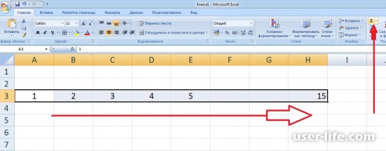
If you need, for example, to check the quantity of all products that are recorded in the table, you can do this by selecting the auto sum icon in the toolbar (it looks like the letter E). After you need to indicate the range of numbers that need to be processed (in this field, all the numbers in the “Quality” field), press Enter - and the program will remove the value. You can also do this manually by selecting all the middles of the “Quality” field and placing a folding sign between them. (= A1 + A2 + ... A10). The result is the same.

How to manage your money in an Excel spreadsheet?
Today we have a theme for the beginnings of the koristuvachs Microsoft Office Excel (Excel), and itself: how to properly organize a sum of numbers?
In fact, Excel is one of the Microsoft Office software packages designed for working with data tables. sum_sna s operating systems Windows and MacOS and software product OpenOffice.

Since Excel (Excel) does not already have ready-made tables with centers for placing data, you can save arithmetic operations in them with groups of data vertically and horizontally, as well as with adjacent centers, or we will label groups of boxes.

Let’s immediately focus on how to grab the bag.
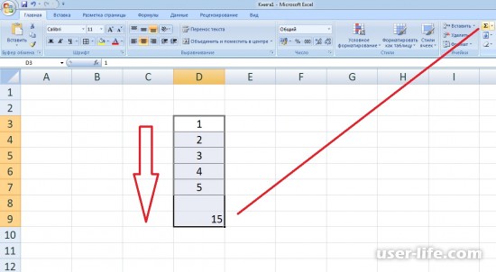
1. You can see the required range of bags with vertical numbers and continue two empty tabs below and press the “Get bag” icon in the program menu.

2. You can see the required range of bags with numbers along the horizontal line two empty tabs below and press the “Get bag” icon in the program menu.

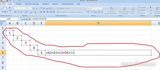
3. You can add the center, spread in different rows and spat. To do this, in Excel you need to select the right position and enter the sum formula. So just (=), select the middle 1+ middle 5+ middle N and press Enter.

Before speaking, you can not only remove the sum, but also multiply, divide, subtract and formulate more complex formulas.

So, right now you need to click the left button of the mouse on any middle and write in it: “= 500 + 700” (without paws). After pressing the “Enter” button, the result will be returned - 1200. The axis is like this in a simple way You can add 2 numbers. In addition to the same function, you can also add other operations - multiplication, division, etc. In this case, the formula will look like this: “number, sign, number, Enter.” This is a very simple example of adding 2 numbers, but, as a rule, in practice it is rarely possible to do this.

hiring;
agility;
price;
sum.
In total in the table there are 5 items and 4 sleepers (all items except sum). The task was set - to know the amount of a leather product.

For example, the first name is a pen: quantity - 100 pieces, price - 20 rubles. To know the amount, you can quickly use this simple formula, once you have already looked at it, then write it like this: “= 100 × 20.” This option is, of course, possible, but it will not be very practical. Let’s say the price of a pen has changed, and now it costs 25 rubles. What should you do - rewrite the formula? And if in the table the names of goods are not 5, but 100 or even 1000? In such situations, Excel can subtract the sum of numbers in other ways, incl. overdo the formula if one of the middle changes.

To grab your bag in a practical way, You will need a different formula. So, from now on you need to put a “dear” sign in the middle of the “Suma” sleeper. Next, you need to click the left mouse button on the number of handles (in this case the number “100”), put the multiplication sign, and then click the left mouse button again on the price of the handle - 20 rubles. After this you can press “Enter”. Then nothing changed, and the result remained unchanged - 2000 rubles.

But there are two nuances here. The first is the formula itself. If you press it on the middle, you can notice that there are not numbers written there, but rather “= B2 * C2”. The program wrote in the formula not to be included, but the names of the middles in which the numbers are found. And another nuance lies in the fact that now, when changing any number in these middles (“Quality” or “Price”), the formula will automatically be overreacted.
If you try to change the price of the pen by 25 rubles, then the usual customer “Suma” will immediately display a different result - 2500 rubles. Then, with this function in place, there is no need to independently reset the skin value if the information has changed. All you have to do is change the output data (if necessary), and Excel will automatically rearrange everything.

After this, the merchant is guilty of seizing the bag and losing 4 titles. For everything, the procedure is carried out in a familiar manner: one sign, a click on the “Kilkist” sign, a multiplication sign, another click on the “Price” and “Enter” sign. ale in Microsoft programs Excel has one very useful function that allows you to save time by simply copying the formula into other fields.

Well, right now you need to see that little box in which the hidden bag of hands was already covered. The middle section will be visible with thick lines, and in the lower right corner there will be a small black square. If it is correct to point the bear at this square, then external look The cursor will be changed: the white “plus sign” will be replaced with a black “plus sign”. At that moment, if the cursor looks like a black plus sign, you need to press the left mouse button on the lower right square and pull it down to the required point (in this case - 4 rows down).

This manipulation allows you to “pull” the formula down and copy it into 4 more layers. Excel will instantly show all the results. If you click on any of these samples, you can see that the program automatically wrote down the required formulas for the skin test and created it absolutely correctly. Such a manipulation will be interesting, since there are already a lot of names in the table. But here there are deeds of exchange.

First of all, the formula can be “pulled” either down/up or to the side (either vertically or horizontally). In another way, the formula is to blame but the same. Therefore, if in one transaction the sum is disbursed, and the next (under it) the numbers multiply, then such manipulation will not help, in this case only a series of numbers will be copied (as the first group was copied).

How can I pay for the additional “AutoSum” function?
Another way to calculate the sum of numbers is through the additional “AutoSum” function. This function should be located in the toolbar (just below the menu bar). “AutoSum” looks like the Greek letter “E”. However, for example, there is a stack of numbers, and it is necessary to know their sum. To do this, you need to see the middle under this column and click the “Autobag” icon. Excel will automatically see all the vertical lines and write the formula, and you won’t have to press “Enter” to edit the result.

If you need to work with hundreds, you'll be glad to know that Excel has tools that can make your task easier.

You can use Excel to maintain your hundreds of thousands of profit and profit indicators. Whether your spending increases or your sales percentage increases from month to month, you will always be aware of the key indicators of your business. Excel will help you with this.

You also learn how to deal with scores on a high level, calculating the arithmetic mean, as well as the percentile value, which can be different in many cases.

Step by step, we will teach you how to insure hundreds of dollars in Excel. Let's take a look at some of the Excel percentage formulas and functions in the application of a worksheet with business expenses and a worksheet with school grades.

You learn the basics that will allow you to easily work with tables in Excel.

demo video

You can marvel outside kerivnitstvo In the demo video or read the detailed description below. To get started, download weekends free files: We will vikoristuvat them in the process of vikonniya rights.

1. Entering data in Excel

Insert the current data (or open the desired file " persentages.xlsx", What is in the initial files of this project). It contains the Expenses sheet. Later we will review the Grades sheet.

Data sheet with hundreds

Insure a large sum

Let’s say that you will see an 8% increase in expenses in the coming year and you want to increase this value.

Before you start writing formulas, it’s worth knowing that in Excel you can work with vikory scales, the 100 sign (20%), and the tens fraction (0.2 or just 2). The widget symbol for Excel does not require any formatting.

We want to increase the amount of money, not just the amount of growth.

Krok 1

In the middle A18 write with 8% for those who grow up. The fragments in the middle are the text and the number, Excel will take into account that the whole middle will replace the text.

krok 2

press Tab, Then in the middle B18 write the following formula: = B17 * 1.08

Or you can use the formula: = B17 * 108%

The sum will be 71.675, as shown below:

Expansion of a large number in Excel

3. Rozrakhunok change in size

Maybe you think that spending will change by 8%. To improve the result, the formula will be similar. Start with showing the actual changed amount, not just the amount of change.

Krok 1

In the middle A19, write 8% for changes.

krok 2

press Tab, Then in the middle B19 write the following formula: = B17 * .92

Or you can write the formula differently: = B17 * 92%

The result will be 61.057.

Rozrakhunok change vіdsotka in Excel

krok 3

If you need the ability to change the size, increase or change the price, then you can write the formulas in the following order:

Formula for growth by 8% in the middle B18 will be = B17 + B17 * 0.08

krok 4

Formula for change by 8% in the middle B19 will be = B17 - B17 * 0.08

In these formulas, you can simply change .08 to any other number to get the result with a different size.

4. Size: 100 cm

Now let's move on to the formula for the breakdown of the size of a hundred. What do you want to know how much to add ci 8%? To earn money, multiply the amount of money in B17 for 8 watts.

Krok 1

In the middle A20 write 8% from the terminal sum.

krok 2

press Tab, I in commerce B20 write the following formula: = B17 * 0.08

Or you can write the formula this way: = B17 * 8%

The result will be 5.309.

Razkhunok size vіdsotka in Excel

5. Making changes without editing formulas

If you want to change the range without editing the formulas, you need to place it in a separate box. Let’s begin with the names of the rows.

Krok 1

Write in the middle A22 Change it. press Enter.

krok 2

Write in the middle A23 the greatest amount. press Enter.

krok 3

Write in the middle A24 Naymensha suma. press Enter.

On Arkusha it may look like the coming order:

Excel sheet with additional rows

Now we will add hundreds and right-hand formulas to the headings.

krok 4

In the middle B22 write 8% . press Enter.

krok 5

In the middle B23 write the next formula that will open up a pouch with an additional 8%: = B17 + B17 * B22

krok 6

In the middle B24 write the following formula that will open up the pouch minus 8%: = B17 * (100% - B22)

Yakscho in the middle B22 If you write 8%, then Excel will automatically format this middle part in the form of hundreds. Whatever you write.08 or 0.08, Excel will save the middle as well. From now on you can change the format of your commercial to the format in the view of hundreds by clicking the button on the page Percent Style:

Percent Style button

Porada: You can format numbers in the hundreds view using an additional key combination Ctrl + Shift +% for Windows or Command+Shift+% for Ma c.

6. Change the size to a hundred

Here's the rule for changing your size:

= (New meaning - old meaning) / new meaning

Since this is the first month, there is no change in the size of the hundred. The first change in the world will be in the fierce, thick with the data of the fierce offensive we will write:

Krok 1

krok 2

Excel display the result as a result, then click the button Percent Style on the page (or use the corresponding key) to display the number in the form of a hundred.

Percent Style button for displaying hundreds of views

Now, if we have hundreds of monthly differences, we can automatically fill in the column with formulas to determine the change in the size of the hundreds for the next month.

krok 3

Point the bear at the required point in the lower right corner of the box, which costs -7%.

Autofill point in Excel

krok 4

If the mouse's indicator changes to a crosshair, sign up double click misha.

If you are not familiar with the autofill function, read about technique 3 in my article about working techniques with Excel:

krok 5

Select a client B3(With the heading "Sum").

krok 6

point bear show on auto-refill point and drag it one square to the right, into the square C3. This way you will duplicate the title at once in its format.

krok 7

In the middle C3 replace title with % Change.

All size changes are fully insured

7. Rozrakhunok vysotka v zagalnyi bag

The remaining technique on this sheet will be the cost of one hundred dollars per month. Display this hundred as a pie chart, set one sector for each month, and set the sum of all sectors to 100%.

It doesn’t matter whether you use Excel or on paper, if you use a simple division operation:

Significance of one element / zagalny sum

I need to present you with a view of the hundred.

In our case, we will divide the monthly amount into the legal amount, which is located at the bottom of column B.

Krok 1

Select a client C3 and sign up autorefill one in the middle, up to D3.

krok 2

Change the text in the middle D3 on % Type of hidden bag.

krok 3

In the middle D4 write this formula until then do not press Enter:=B4/B17

krok 4

Before pressing the enter key, we need to re-convert so that there will be no reprieve during auto-fill. We will automatically fill the columns down with the fragments, the dealer (infection with B17), is not obliged to change. Even if you change, then all the changes from fierce to the chest will appear incorrect.

Check again to see that the text cursor is still in the middle before the “B17” section.

krok 5

press F4(On Mac - Fn+ F4).

So you insert a dollar sign ($) in front of the column and row values, and the value will appear as follows: $B$17. $B means that column B will not change to column C, etc., but $17 means row number 17 will not change to row 18 etc.

krok 6

Check out what the resulting formula looks like: =B4/$B$17.

Formula for vysotka v zagalnyi sumi

krok 7

Now you can press the Enter key and select autofill.

press Ctrl + Enter(On Mac - Command+ ↩) to enter the formula without moving the mouse cursor into the middle below.

krok 8

Press button Percent Style on the page or use the same keys Ctrl+ Shift+ % (Command+ Shift+ %).

krok 9

Point the mouse cursor above the auto-fill point in the middle D4.

krok 10

When the cursor changes to a crosshair, click on double click please, to automatically fill the middles below with formulas.

Now, for each month, the value of your monthly sum will be displayed.

Replenishment of hundreds of items in the legal bag

8. Percentage ranking

The ranking value is expressed as a percentage using a statistical method. You, melodiously, are familiar with it from schools, when the average score of students is calculated, and this allows them to be ranked according to their appearance. The higher the rating, the higher the number.

The list of numbers (ratings, in our version) is located in the group of middles, which in Excel are called an array. The massifs have nothing special, so let’s not give them any significance. Excel simply names the range of values ​​that you use in the formula.

Excel has two functions for calculating percentage rankings. One of them includes the cob and tail values ​​of the array, and the other does not.

Marvel at another sheet bookmark: Grades.

Percentage ranking in Excel - sheet with ratings

Here is a list of 35 average points, sorted by age. First, what we want to know, this percentage is not ranked for the average skin score. For this purpose we will use the function = PERCENTRANK.INC. "INC" in this function means "inclusive", which will include the first and last items in the list. If you want to turn off the first and second array, then use the function = PERCENTRANK.EXC.

The function has two common arguments and looks like this: = PERCENTRANK.INC(array, entry)

• array(Array) - this is a group of middle ones that make up a list (in our version B3:B37)
• entry(Value) - whether it is significant or the middle in the list

Krok 1

Select the first item in the list C3.

krok 2

Write the next formula, do not press the Enter key:=PERCENTRANK.INC(B3:B37

krok 3

This range must remain unchanged so that we can stop auto-refilling all the middle parts down.

So press the key F4(On Mac - Fn+ F4), Add the dollar sign to the value.

The formula is to blame for the upcoming rank: = PERCENTRANK.INC ($B$3:$B$37

krok 4

In the skin center in column C, we have an important percentage ranking of the specific value in the column B.

Press onto the middle B3 and close the arms.

The formula in the pouch is: =PERCENTRANK.INC ($B$3:$B$37,B3)

Percentage ranking function

Now we can enter and format the values.

krok 5

If necessary, select the middle again C3.

krok 6

visconite double click target on Automatic filling point middles C3. This will automatically fill the middle of the column lower.

krok 7

On the page, press the button Percent Style, To format the column in the hundreds view. As a result, you are responsible for hurting your feet:

The formatted percentage ranking function has been added

So, if you have good grades and your GPA is 3.98, then you are in the 94th percentile.

9. Calculation of percentile.

Using the PERCENTILE function, you can expand the percentile. For this additional function, you can enter the size of the panel and subtract the values ​​from the array that represent the panel. Since there is no exact value in the range, Excel will show those values ​​that are in the list.

In what types of seizures is this necessary? For example, if you are applying to a university program that only accepts students who fall within the 60th percentile. And you need to find out which average score corresponds to 60%. Having marveled at the list, we are surprised that 3.22 is 59%, and 3.25 is 62%. Vikorist function = PERCENTILE.INC we recognize the exact confirmation.

The formula will be like this: = PERCENTILE.INC (array, percent rank)

• array(Array) - this is a range of items that make up a list (as in the previous example, B3:B37)
• rank(Rank) - hundreds of hundreds (or tens of units from 0 to 1 inclusive)

Just like for the percentage ranking function, you can use the function = PERCENTILE.EXC, which includes the first and remaining values ​​of the array, but in our example this is not necessary.

Krok 1

Select under the list of middles B39.

krok 2

Insert the following formula into it: = PERCENTILE.INC (B3: B37.60%)

So, since we don’t need to stagnate the auto-replacement system, there is no need to work on the unchangeable array.

krok 3

Press the key once on the page Decrease Decimal(Change the digit) to round the number to two tenth digit after the coma.

As a result, in this array the 60th percentile will be the average score of 3.23. Now you know what assessments are required in order to be accepted into the program.

The result of the calculation percentile function

visnovok

The hundreds are not complicated at all, and Excel develops them, using the same rules of mathematics as you would if you were reading them on paper. Excel also shows the basic order of operations in these cases, if your formula has addition, substitution, and multiplication:

1. temples
2. Indicator stage
3. multiplication
4. split up
5. additional
6. vidnіmannya

I remember this order using an additional mnemonic phrase: Sk Azal st epan: roseum ora, D Let's sl OVIMU IN ora.

Most beginners often wonder about nutrition - how to quickly get hundreds of dollars in Excel or what formula is best to quickly deal with degeneration.

It is not possible to take a certain time under the founded rosrahuki, it is cleanly cleaned by the oscillator consuming the wire in the store I. Zakinchoi, they are with accounting rosrahuks, such, Yak Voznoye Sumi, Yaku Slid Vislatti for clans.

Zmist:

breakdown of hundreds of units

Varto begins with the fact that the formula for the breakdown of hundreds of hundreds differs from the mathematical one we know. She looks out at the coming rank:

Part / Cile = Vidsotok

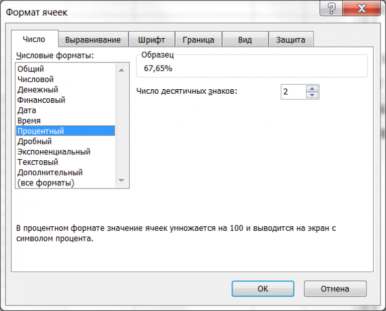
Dear correspondent, please note immediately that the multiplication by 100 is not calculated and there will be proper respect. The only axis in the program is not required if you set the middle "Percentage format", The program will be delivered independently. Now let's look at all the necessary actions on the butt.

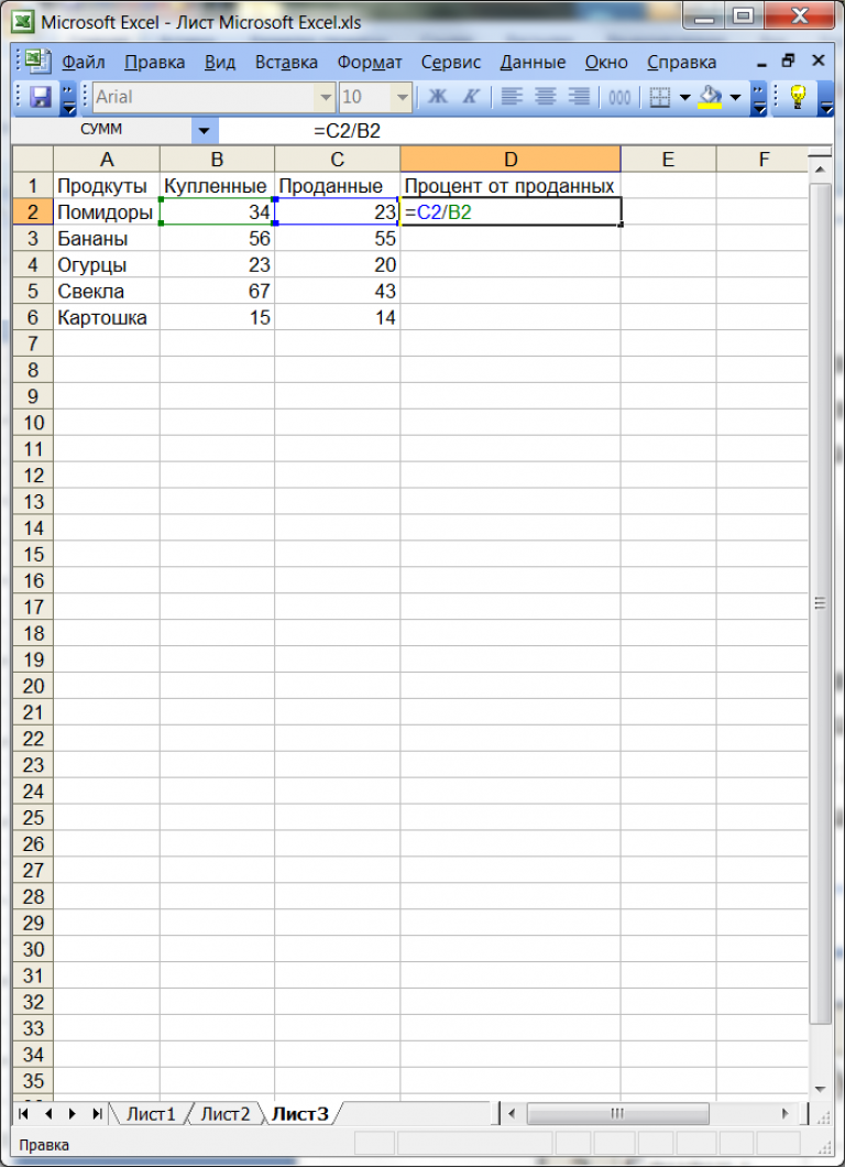
Let’s assume that we have a list of products (section A) and data on them - how many were previously purchased (section B), and how many of them were subsequently sold (section C).

It is important for us to know what type of purchased goods are included in sales (section D). For whose sake we need to step:

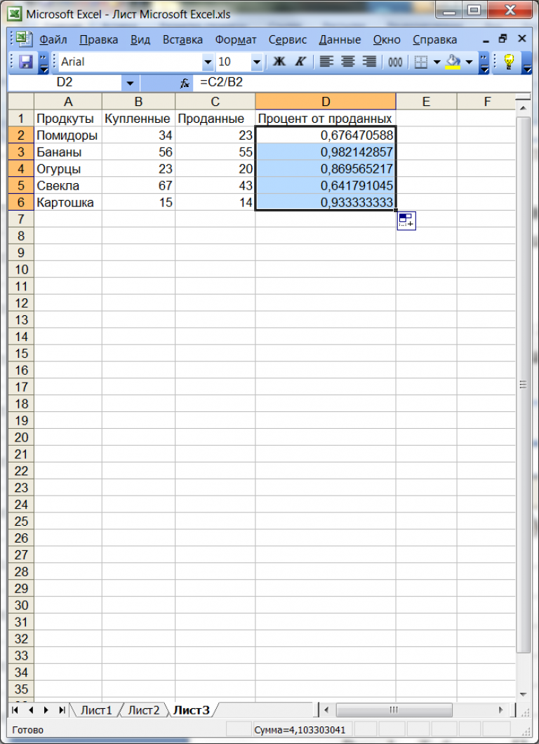
• We enter the formula = C2 / B2 into the middle D2, and in order not to work too much with the rows, simply select the auto-fill marker and copy them down onto the insoles, as many as necessary.