Filter with end-to-end impulse characteristic. Feeding. Digital filters with end-of-line impulse response (ICR) With end-of-end impulse response
End-to-end impulse response filter (Non-recursive filter, KIX filter) or FIR filter (FIR speed as a finite impulse response - end-impulse characteristic) - one of the types of linear digital filters, the characteristic feature of which is that the impulse characteristic is aligned with the hour (at which point the hour becomes exactly equal to zero). Such a filter is also called non-recursive due to the presence of a gateway link. The symbol of the transfer function of such a filter is a constant.
Dynamic characteristics
de - delta function. The impulse response of the FIX filter can be written as:
#define N 100 // Filter order float h [N] = ( #include "f1.h"); //Insert a file with known filter coefficients float x [N]; floaty[N]; short my_FIR(short sample_data) ( float result = 0 ; for ( int i = N - 2 ; i >= 0 ; i-- ) ( x[ i + 1 ] = x[ i] ; y[ i + 1 ] = y[i];) x[0] = (float) sample_data;for (int k = 0; k< N; k++ ) { result = result + x[ k] * h[ k] ; } y[ 0 ] = result; return ((short ) result) ; }
Div. also
Posilannya
- Design of an FIR filter with a linear phase-frequency characteristic using the frequency sampling method
Wikimedia Foundation. 2010.
- Romodin, Volodymyr Oleksandrovich
- Vokhma (river)
See also “Filter with end-to-end impulse response” in other dictionaries:
Filter - pick up the current BeTechno promotional code at the Academy or you can easily buy a filter at a discount on sales at BeTechno
end-impulse response filter- - Topics of electrical signals, basic concepts EN finite impulse response (filter) FIR ... Adviser of technical translation
Filter with unskewed impulse response- (Recursive filter, BIX filter) or IIR filter (IIR speed.
KIX filter
Non-recursive filter- A filter with an end-of-line impulse response (non-recursive filter, FIR filter, FIR filter) is one of the types of linear electronic filters, the characteristic feature of which is that it is connected to the hour of its impulse response (with what... Wikipedia
Recursive filter- A filter with an unskewed impulse characteristic (Recursive filter, BIR filter) is a linear electronic filter that uses one or more of its outputs as an input, so that it eliminates the return link. The main power of such filters is ... Wikipedia
Digital filter- A digital filter in electronics is a filter that processes a digital signal to detect or suppress the low frequencies of its signal. In the digital mode, the analog filter is located to the right of the analog signal, which has power.
Discrete filter- A digital filter in electronics is a filter that processes a digital signal to detect or suppress the low frequencies of its signal. On view, the digital analog filter is located to the right of the analog signal, whose power is non-discrete, ... Wikipedia
Line filter- Linear filter is a dynamic system that freezes any linear operator before the input signal in order to see or suppress high frequencies of the signal and other processing functions of the input signal. Linear filters are widely used in ... Wikipedia
Kovzna serednya (filter)- Which term has other meanings, div. Serednya kovzna (meaning). Block diagram of a simple KIK filter of a different order, which implements a cross-median, a cross-median, a cross-median type of digital filter with ... Wikipedia
Meaningful mean (meaning)- Moving average, moving average: Moving average is a family of functions whose values at the skin point are equal to the average value of the output function for the forward period. Sliding average... ... Wikipedia
Let's look at the simplest of digital filters - filters with constant parameters.
The digital filter receives an input signal that looks like a sequence of numerical values at intervals (Fig. 4.1, a). When the skin core value is matched to the digital filter signal, the skin core value of the output signal is decomposed. The decomposition algorithms may be very different; During the expansion process, the remaining values of the input signal may be subject to change
Foremost values of input and output signals: The signal at the output of the digital filter is also a sequence of numerical values that are output at intervals. This interval is the same for the digital signal processing device.

Rice. 4.1. Signal at the input and output of the digital filter
Therefore, apply the simplest signal in the form of a single pulse to the input of the digital filter (Fig. 4.2 a)
![]()
then the output is a signal that looks like a discrete sequence of numerical values that accumulate over an interval
In analogy with basic analog lanyards, this signal is called the impulse response of the filter (Fig. 4.2, b). Based on the impulse characteristics of the analog lanyard, the function is dimensionless.

Rice. 4.2. Single pulse and impulse response of a digital filter
A sufficiently small discrete signal is supplied to the filter input. 4.1 a), which is a set of discrete values
Under the action of the first element at the output of the filter, the sequence is formed multiplied by when the sequence is multiplied by and pushed to the right by the amount, etc. As a result, the sequence is taken out at the output

Thus, the output signal is defined as a discrete sample of the input signal and impulse response. Its advanced digital filters are similar to those of conventional lancets, where the output signal is similar to the input signal and impulse characteristics.
Formula (4.1) is a digital filtering algorithm. Since the impulse response of the filter is described in sequence with the end number of terms, the filter can be implemented in the form of the circuit shown in Fig. 4.3. Here the letters indicate the elements of the time-clock signal (one in the middle); -elements to multiply the signal by the positive coefficient
The diagram is shown in Fig. 4.3 does not contain the electrical circuit of the digital filter; This diagram is a graphical representation of the digital filtering algorithm and shows the sequence of arithmetic operations that are completed when processing the signal.

Rice. 4.3. Non-recursive digital filter circuit
For digital filters that process signals as abstract numerical sequences, the concept of “clockwise shading” is not very correct. Therefore, the elements that interfere with the signal per channel are indicated on digital filter diagrams with a symbol that indicates the blocking of the signal - reshaping. We have reached the end of this purpose.
Let's return to the digital filter circuit shown in Fig. 4.3 Such filters, which are used for decomposition based on the value of the input signal, are called simple or non-recursive.
The non-recursive filter algorithm is easy to write based on the impulse response of the filter. For practical implementation of the algorithm, it is necessary that the impulse characteristic meets the end number of terms. Since the impulse characteristic has an infinite number of members, but it changes quickly over the value, you can limit the number of members by adding some values. If the elements of the impulse response do not fall off with value, the non-recursive filter algorithm becomes unrealizable.

Rice. 4.4. -lanzug
As a butt, let’s look at the simplest digital filter, similar to the Lantzug (Fig. 4.4). The impulse characteristic of the Lanzug is visible
![]()
To record the impulse response of a reliable digital filter, replace the expression with However, the impulse response of a lancet has dimensions, and the impulse response of a digital filter must be dimensionless. Therefore, we omit the multiplier in the form (4.2) and write the impulse response of the digital filter in the form
![]()
Such an impulse characteristic has an infinite number of members, but its value changes according to the exponential law, and it is possible to exchange members, choosing such that
Now you can record the value of the signal at the filter output
This is done simultaneously by a digital filter algorithm. The diagram of this filter is shown in Fig. 4.5.
Another approach to the analysis of processes in digital filters is similar to the operator method of analyzing primary analogues, but instead of the Laplace transformation, the vicorist transformation is used.

Rice. 4.5. Scheme of a non-recursive digital filter, similar to the Lantzug
What is significant is the digital filter parameter, which is similar to the transfer function of an electric lancet. For this purpose, it is necessary to transform the impulse characteristics of the digital filter:

The function is called the system filter function.
Corresponding to expression (4.1), the signal at the output of the digital filter is similar to the discrete group of the input signal and the pulse characteristics of the filter. Having established the theorem about the transformation of the throat to this extent, we can reject that the transformation of the output signal is the same as the transformation of the input signal, multiplied by the system filter function:
![]()
Thus, the system function plays the role of the transfer function of the digital filter.
As a matter of fact, we know the system function of a first-order digital filter, similar to a lancet:

The third method of analyzing the passage of signals through digital filters is similar to the classic method of differential measurements. Let's take a look at this method in order.
The simplest analogue lancet of the 1st order is the e-lancug (div. Fig. 4.4), the passage of signals through it is described by differential levels
![]()
For a discrete lancer, instead of the differential level (4.8), the differential level is recorded, where the input and output signals are specified for discrete moments of the hour, and instead of the corresponding one, the difference of the constant values is determined No signal. For a discrete Lanzug of the 1st order, the divisional level can be written down in the official form
It will stagnate until it is re-created
We know the system filter function
![]()
Formula (4.10) is a basic expression for the system function of a 1st order digital filter. In this case, we avoid the previously removed expression (4.7) for the system function of a digital filter, equivalent to a lancet.
We know the digital filtering algorithm, which corresponds to the system function (4.10). For whom is jealousy (4.9) good?
An equivalent diagram of this algorithm is shown in Fig. 4.6. The equation with a non-recursive filter (div. Fig. 4.5) has a kind of “reversible linkage”, which means that the value of the output signal is vicorized in the next step

Rice. 4.6. Scheme of a recursive digital filter, similar to the Lantzug
rozrahunkah. Filters of this type are called recursive.
Algorithm (4.11) provides a filter that is essentially equivalent to the non-recursive filter discussed earlier. If one value of the output signal is obtained using the non-recursive filter algorithm (4.4), one operation is required, and the recursive filter algorithm (4.11) requires two operations. This is the main advantage of recursive filters. In addition, recursive filters allow signal processing to be carried out with greater accuracy, which allows them to more correctly implement the impulse response without removing the “tail”. Recursive filters allow you to implement algorithms that otherwise cannot be implemented using non-recursive filters. For example, with a filter, which follows the circuit in Fig. 4.6, in essence, an ideal accumulator-integrator has an impulse characteristic of the form. A filter with such a characteristic cannot be implemented in a non-recursive circuit.
The examples reviewed show that there is no sense in using non-recursive algorithms for creating digital filters with a long impulse response. In these cases, recursive filters are more powerful.
The area of application of non-recursive algorithms is the implementation of digital filters with an impulse response, which allows for a small number of members. An example could be a simple differentiator, the output signal being equal to the increase in the input signal:
The diagram of such a digital filter is shown in Fig. 4.7.

Rice. 4.7. Circuit of the simplest digital differentiator
Let's now take a look at the digital filter, which is described by our peers
The equation can be seen both as a retail order and as a digital filtering algorithm, which can be rewritten differently, and also as a digital filtering algorithm.

Rice. 4.8. Digital recursive filter circuit in order
Algorithm (4.13) is supported by the diagram shown in Fig. 4.8. We know the system function of such a filter. For which it is necessary to stagnate and recreate:
Viraz (4.14) allows you to establish connections between the elements of the filter circuit and the system function. The coefficients in the system function numeric mean the values of the coefficients at
(At the non-recursive part of the filter), and the coefficients in the banner indicate the recursive part of the filter.
NOVOSIBIRSK STATE TECHNICAL UNIVERSITY
FACULTY OF AUTOMATION AND VICHIVAL TECHNOLOGY
Department of Data Collection Systems
Discipline “Theory and signal processing”
Laboratory robot no.10
DIGITAL FILTERS
WITH END IMPULSE CHARACTERISTICS
Group: AT-33
Variation: 1 Vikladac:
Student: Shadrina A.V. Assoc. Shchetinin Yu.I.
Meta robots: development of methods for analysis and synthesis of filters with end-impulse characteristics and vicarious end-to-end functions that are smoothed.
Vikonannya roboti:
1. Graphs of the impulse response of a low-pass FIX filter with a direct-window frequency section for the filter's maximum value.
The impulse response of an ideal discrete FIX filter is unskewed and not equal to zero for negative values:
 .
.
To remove a physically active filter, surround the impulse response with an end number, which will destroy the truncated response to the right value.
The value is the size (size) of the filter, ![]() - Filter order.
- Filter order.
Matlab Script (labrab101.m)
N = input("Enter filter date N = ");
h = sin(wc.*(n-(N-1)/2))./(pi.*(n-(N-1)/2));
xlabel("Video number, n")
>> subplot(2,1,1)
>> labrab101
Enter filter value N = 15
>> title("Impulse response of the KIX filter for N=15")
>> subplot(2,1,2)
>> labrab101
Enter filter value N = 50
>> title("Impulse response of the KIX filter for N=50")

Fig.1. Graphs of the impulse response of a low-pass FIX filter with a direct-window frequency section for the maximum value of the filter
Comment: How to look at the frequency response of a digital filter as a Fourth series:  , then the coefficients of this series will be the values of the impulse characteristic of the filter. In this phase, the low Four'e was truncated in the first phase to , and in the other – to , and then the truncated characteristics were inserted along the axis of the right hand to remove the causal filter. When the width of the head cap is set to 2, and when - 1, then. With a larger filter, the impulse response control will sound. If you look at the rhubarb of wild pellets (for help), then with increased wine, the absolute value increases to . In this way, it is possible to create a system so that with a vicoristic approximation of the ideal frequency response of a filter with a straight-cut window, it is not possible to simultaneously sound the head pellets (and thereby change the transition region) and change the levels of the horn pellets (change sew pulsations in filter transmission and filtration). A single ceramic parameter of a rectangular window is its size, in addition to which you can inflate the width of the head pellet, but on the side pelust there is no special infusion.
2. Calculation of the DVPF of impulse characteristics from clause 1 for an additional function. Graphs of their frequency response on a linear scale and in decibels 512 Vіlіkіv frequencies. Transmission smudge, transition smudge and filter smudge. Infusing the order of the filter into the width of the transitional smudge and the level of pulsation of the frequency response in the smug of transmission and trimming.
Matlab Function (DTFT.m)
function = DTFT(x,M)
N = max(M, length(x));
% Reduced FFT to size 2^m
N = 2^(ceil(log(N)/log(2)));
% Calculation fft
% Frequency vector
w = 2*pi*((0:(N-1))/N);
w = w - 2 * pi * (w> = pi);
% Zsuv FFT to interval from -pi to +pi
X = fftshift(X);
w = fftshift(w);
Matlab Script (labrab102.m)
h1 = sin(wc.*(n1-(N1-1)/2))./(pi.*(n1-(N1-1)/2));
h2 = sin(wc.*(n2-(N2-1)/2))./(pi.*(n2-(N2-1)/2));
DTFT(h1,512);
DTFT(h2,512);
plot(w./(2*pi),abs(H1)./max(abs(H1)),,"r")
xlabel("f, Hz"), ylabel("|H1|/max(|H1|)"), grid
plot(w./(2*pi),abs(H2)./max(abs(H2)),,"b")
xlabel("f, Hz"), ylabel("|H2|/max(|H2|)"), grid
plot(w./(2*pi),20*log10(abs(H1)),,"r")
title("Frequency response of a low-pass FIX filter with a straight-cut window for N = 15")
xlabel("f, Hz"), ylabel("20lg(|H1|), dB"), grid
plot(w./(2*pi),20*log10(abs(H2)),"b")
title("Afrequency response of a low-pass FIX filter with a straight-cut window for N = 50")
xlabel("f, Hz"), ylabel("20lg(|H2|), dB"), grid

Fig.2. Frequency response graphs of a low-pass FIR filter with a rectangular window frequency, plotted for the filter value and on a linear scale

Fig.3. Frequency response graphs of a low-pass FIR filter with a straight-cut window frequency plotted for the filter input value on a logarithmic scale
Comment:
Table 1. Range of transmission smudge, transition region and back-up smudge for the filter value
|
Filter refill |
Smuga transmission, Hz |
Transition region, Hz |
Smuga of back-up, Hz |
||||||||||||||||||||||||||||||||||||||||||||||||||||||||
|
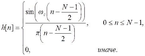
Lecture No. 10 "Digital filters with end-to-end impulse response" The transferred function of the digital filter, which is physically implemented, with the end-impulse characteristic (FIR filter) can be presented in the form (10.1). When replacing the view (10.1), the frequency response of the FIX filter is removed from the view de Phase trimming filter is indicated as Group grooming filter is indicated as An important feature of KIKh filters is the ability to implement the effects of stable phase and group blocking, etc. linear phase response (10.5), de a - Constant. When the filter is filtered, the signal that passes through the filter does not change its shape. To clear the minds to ensure linear phase response, we write down the frequency response of the FIR filter with equation (10.5) Equivalent actions and obvious parts of this equality are rejected Having shared equal feelings with each other, we reject The remainder can be written There are two decisions to be made. Perche at a =0 indicates jealousy The whole process has a single solution, which is satisfactory h (0) (sin (0)=0), і h (n)=0 at n >0. This solution corresponds to a filter whose impulse characteristic has a single non-zero output at the beginning of the hour. This filter is of practical interest. We know another solution for . With this, having cross-multiplied the numerals and the signifiers (10.8), we can eliminate (10.11). Zvidsi maemo The ruins of the village look like a low Four'e, his decision, as it is, is the only one. It is easy to note that the result of this jealousy can influence the minds (10.13), (10.14). 3 minds (10.13) is pouring out, which is a filter for the skin N There is only one phase delay a , for which the strict linearity of the phase response of the mind (10.14) can be achieved, it follows that the impulse response of the filter may be symmetrical to the point for the unpaired N , that is, to the middle point of the interval (Fig. 10.1).
The frequency response of such a filter (for unpaired N ) can be written down on view (10.15). Roblyachi in another amount replacement m = N -1- n, eliminated (10.16). Shards h (n) = h (N-1-n ), then the two sums can be combined Substituted, rejected (10.18). What do you mean? then the remainder can be written Thus, for a filter with a linear phase response it is possible For a doubles match N similar to mathemo Costly replacement in another amount will be withdrawn Robly replacement, discarded (10.24). Having signified we will have the rest of the mother In this way, for a FIX filter with a linear phase response, the same order N can be written Below, for the sake of simplicity, we can only see filters with an unpaired order. When synthesizing the transfer function of the filter, the output parameters are related to the frequency response. There are many methods for the synthesis of NIX filters. Let's take a look at their actions. Since the frequency response of any digital filter is a periodic function of frequency, it can be seen as a low Fourier de koefіtsієnєtsya row Fur'є rіvni It is clear that the coefficients are low. h(n ) are avoided with the coefficients of the impulse characteristics of the filter. Therefore, if you have an analytical description of the required frequency response of the filter, you can easily determine the coefficients of the impulse response, and from them, the transfer function of the filter. However, in practice this is not realized, since the impulse characteristic of such a filter is subject to endless repayment. In addition, such a filter is not physically feasible, since the impulse response begins at -¥ , and even the final trim does not make this filter physically implementable. One of the possible methods for deriving a FIR filter that approximates a given frequency response lies in the truncated uncut Fouret series of the impulse response of the filter, importantly h (n) = 0 at . Todi Physical implementation of the transfer function H(z ) can be reached by the path of multiplication H(z) on . de (10.32). With such a modification of the transfer function, the amplitude characteristic of the filter does not change, but the group blocking increases by a constant amount. As a butt, we open up the FIX low-pass filter based on the frequency response of the form Exactly up to (10.29) the coefficient of impulse characteristics of the filter is described by the expression Now (10.31) you can remove the expression for the transfer function de (10.36). Amplitude characteristics of a rated filter for different types N presented in Fig. 10.2.
Fig.10.2 The pulsations in the transmission and distortion are due to the increasing frequency of the low Fourier, which, in turn, is due to the growth of the function at the frequency of the transmission. These pulsations are visible as Gibbs pulsations. From Fig. 10.2 it is clear that this increase N the pulsation frequency increases, and the amplitude changes, both at lower and higher frequencies. However, the amplitude of the remaining pulsation in the smoothie throughput and the first pulsation in the smoothie is almost unchanged. In fact, such effects are often unforeseen, which is due to the reduction of Gibbs pulsation. Enhanced impulse response h(n ) it is possible to create the necessary unstrained impulse characteristics and actions window functions w (n) dovzhini n (Fig. 10.3).
In the considered case of a simple truncated series, Four'e is vikorist directly In this case, the frequency response of the filter can be represented in the form of a complex filter This means that it will be a “shredded” version of the required characteristic. The task is to search for the function of the window, which allows you to change the Gibbs pulsation at the same time as the filter vibrancy. And it is necessary to learn from the beginning the power functions of the window from the butt of the straight-cut window. The spectrum of the function of a straight-cut window can be written as spectrum of the function of the rectangular window of representations in Fig. 10.4.
Fig.10.4 If fragments are present, then the width of the head spectrum spectrum appears equal. The presence of biological pellets in the range of the window function is caused by an increase in Gibbs pulsation in the frequency response of the filter. To remove small pulsations from the smoothie, the transmission and great extinction of the smoothie is necessary so that the area surrounded by the head pellets becomes a small part of the area surrounded by the head pellets. In its own way, the width of the head plate determines the width of the transition zone of the filter, which results. For high filter vibrancy, the width of the head plate may be as small as possible. As can be seen from the deposit, the width of the head pellet changes with increasing filter order. Thus, the power of the various functions of the window can be formulated as follows: - The window function may be limited to the hour; - The spectrum of the window function is due to the best approximation of the function, separated by frequency, then. there is a minimum of energy between the main core; - The width of the main part of the spectrum of the eyelid function is due to its small capacity. The most commonly used functions are: 1. Straightforward. Looked further. 2. Hamming's window. de. In which case the window is called the Henna window ( hanning). 3. Blackman's window. 4. Bartlett's window. The indicators of filters generated by the settings of the functions of the windows are shown in Table 10.1.
The pulsation coefficient is calculated as the ratio of the maximum amplitude of the barrel pellet to the amplitude of the head pellet in the spectrum of the window function. To select the required filter order and the most suitable function of the window during the development of real filters, you can use the data in Table 10.2.
As can be seen from Table 10.1, there is a significant relationship between the coefficient of pulsation and the width of the head pellet in the spectrum of the eyelid function. The smaller the pulsation coefficient, the larger the width of the head pellet, and therefore the transition zone in the frequency response of the filter. To ensure low pulsation in the smoothie throughput, you must select a window with a suitable pulsation coefficient, and the required width of the transition zone is ensured by the advanced filter order N. This problem can be seen in the following window, provided by Kaiser. The Kaiser window function can be viewed
where a is an independent parameter,
The added power of the Kaiser window is the ability to smoothly change the pulsation coefficient from small to large values by changing just one parameter a. In this case, as for other window functions, the width of the headband can be adjusted by filter order N. The main parameters that are set when developing a real filter are: Smuga throughput - w p; Smuga fenced - w a; The maximum permissible pulsation of a smoothie throughput is A p; Minimal loss in smoothies – A a; -sampling frequency - w s. These parameters are illustrated in Fig. 10.5. When the maximum pulsation of a smoothie, the throughput is determined as
and minimally extinguished in the smoothie as The very simple procedure for developing a Kaiser filter filter includes the following steps: 1. The impulse response of the filter h (n) is determined, the frequency response is ideal
de (10:49). 2. Select parameter d as
de 3. The reference values A a and A p are calculated using formulas (10.46), (10.47). 4.Select parameter a as
5.Select parameter D as
6. Select the least important filter order in mind
screams, what The fragments of the impulse characteristics of the filter and the coefficients of its transfer function, mind (10.59) means that the codes of all coefficients of the filter contain only the fractional part and the sign digit and take revenge on the whole part. The number of discharges of the shot part of the filter coefficients is determined by the satisfaction with the transfer function of the filter with quantized coefficients, which can be used to approach the reference transfer function with exact values of coefficients. The absolute values of the input signals of the filter are standardized so that If the analysis is carried out for a FIX filter with a linear phase response, then the algorithm for calculating the output signal can be applied de - Rounded to s k filter coefficient. This algorithm is supported by the block diagram of the filter, which is shown in Fig. 10.5.
There are two ways to implement this algorithm. In the first phase, all operations are multiplied exactly and rounded up on a daily basis. And here the capacity of the creation is the same as s in + s k, where s in is the capacity of the input signal, and s k is the capacity of the filter coefficients. And here the block diagram of the filter, shown in Fig. 10.5, exactly matches the real filter. With another method of implementing algorithm (10.61), the result of the operation is multiply rounded, then. creations are counted with a song of destruction. In this case, it is necessary to change the algorithm (10.61) so as to avoid the loss that is introduced, rounding the creations Since the values of the output signal of the filter are calculated using the first method (with the exact values of the output), then the dispersion of the output noise is calculated as
tobto. lie in the dispersion of the rounding noise of the input signal and the value of the filter coefficients. Here you can find out the required number of discharges of the input signal as
Using the given values of s in and s k, you can determine the number of discharges required for the shot part of the output signal code. Since the values of the output signal are calculated in a different way, if the output is rounded to s d digits, then the dispersion of the noise of the rounding generated by the multiples can be expressed through the digit of the addition DR in is the signal-to-noise ratio at the filter output SNR out . The value of the dynamic range of the input signal in decibels is calculated as
where A max and A min are the maximum and minimum amplitude of the filter input signal. The signal-to-noise ratio at the filter output, expressed in decibels, is expressed as
means the root mean square value of the intensity of the output sinusoidal filter signal with amplitude A min, and (10.77) indicates the reduction of noise at the filter output. 3 (10.75) and (10.76) at A max =1 we can determine the dispersion of the noise output filter The value of the dispersion of the filter's output noise can be calculated to calculate the capacity of the input and output signals of the filter. | |||||||||||||||||||||||||||||||||||||||||||||||||||||||||||
 (10.7).
 (10.8).
 (10.9).
 (10.10).

 (10.17).
 (10.19),
 (10.20).
 (10.21).
 (10.22).
 (10.23).
 (10.26).
 (10.27).
 (10.29).
 (10.30).
 (10.31),
 (10.33).
 (10.34).
 (10.35),


 (10.38).
 (10.39).
 (10.40).

 (10.41),
 (10.42).
 (10.43).
 (10.44),
 (10.45).
 (10.51).
 (10.52).
 (10.53).
 (10.57)
 (10.67).